
Machine Learning models are great and powerful. However, the usual characteristics of regular training can lead to serious consequences in terms of security and safety. In this blog post we will take a step back to revisit a regular optimization problem using an example of a binary classification. We will show a way to create more robust and stable models which use features that are more meaningful to humans. In our experiments we will do a simple binary classification to recognize the digits zero and one from the MNIST dataset.
Firstly, we will introduce why regular training is not perfect. Next, we will briefly sum up what regular training looks like, and then we will outline more robust training. Finally, we will show an implementation of our experiments and our final results.
Overview
Machine Learning models have achieved extraordinary results across a variety of domains such as computer vision, speech recognition, and natural language modeling. Using a training dataset, a model looks for any correlations between features that are useful in predictions. Every deep neural network has millions of weak patterns, which interact, and on average, give the best results. Nowadays, models in use are huge regardless of the domain e.g. the Inception-V4 (computer vision) contains around 55 million parameters, the DeepSpeech-2 (speech recognition) over 100 million parameters, or the GPT-2 (NLP language model) over 1.5 billion parameters. To feed such big models, we are forced to use unsupervised (or semi-supervised) learning. As a result, we often end up with (nearly) black-box models, which make decisions using tons of well-generalized weak features, which are not interpretable to humans. This fundamental property can lead to severe and dangerous consequences in the security and safety of deep neural networks in particular.
Why should we care about weak features? The key is that they are (rather) imperceptible to humans. From the perspective of security, if you know how to fake weak features in input data, you can invisibly take full control of model predictions. This method is called an adversarial attack. This is based on finding a close perturbation of the input (commonly using a gradient), which crosses the decision boundary, and changes the prediction (sometimes to a chosen target, called targeted attacks). Unfortunately, most of the state-of-the-art models, regardless of the domain (image classification, speech recognition, object detection, malware detection), are vulnerable to this kind of attack. In fact, you do not even need to have access to the model itself. The models are so unstable that a rough model approximation is enough to fool them (transferability in black-box attacks).
Safety is another perspective. Our incorrect assumption that training datasets reflect a true distribution sometimes comes back to haunt us (intensified by data data poisoning). In deep neural networks, changes in distribution can unpredictably trigger weak features. This usually gives a slight decline in performance on average, which is fine. However, this decrease often comes as a result of rare events, in which the model will without a doubt offer wrong predictions (think about incidents regarding self-driving cars).
Regular Binary Classification
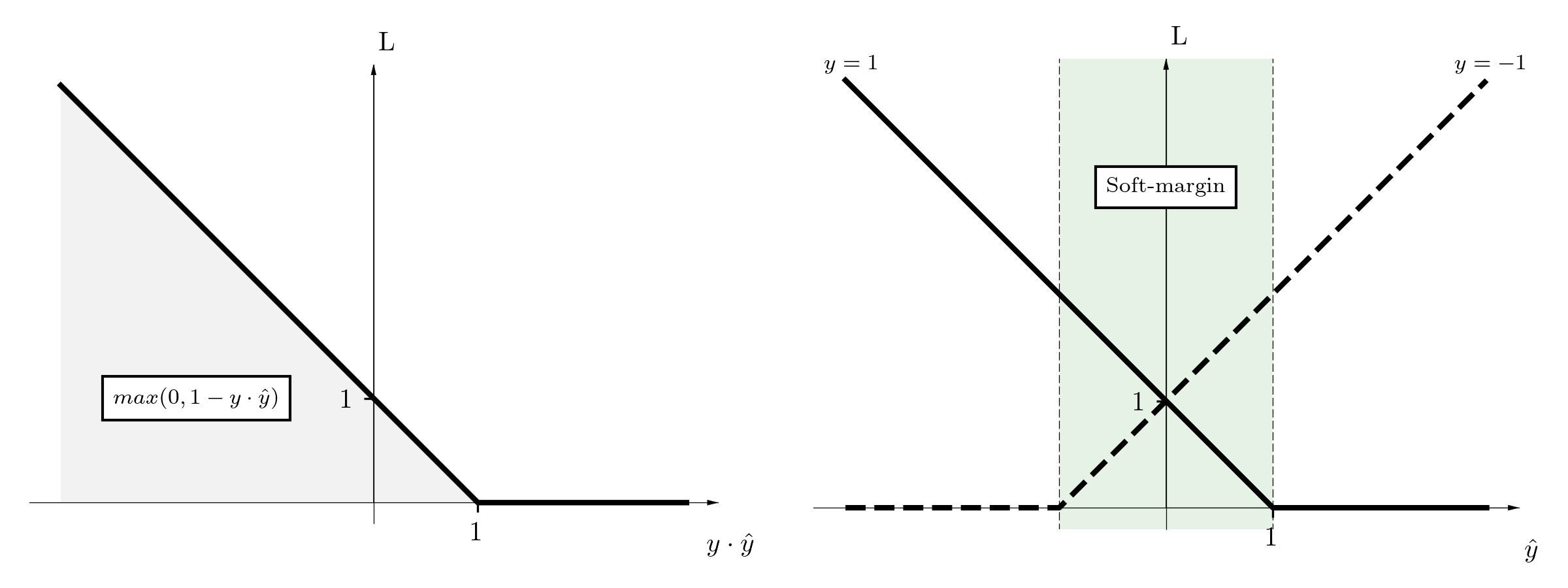
Let’s summarize a regular training procedure. A model, based on some input, makes a hypothesis \(\hat{y} = h_{\theta}(x)\) to predict the correct target \(y\), where \(y \in \{ -1, 1\}\) is in the binary classification. The binary loss function can be simplified to the one-argument function \(L(y \cdot \hat{y})\), and we can use the elegant hinge loss, which is known as the soft-margin in the SVM. To fully satisfy the loss, the model has to not only ideally separate classes but also preserve a sufficient margin between them.
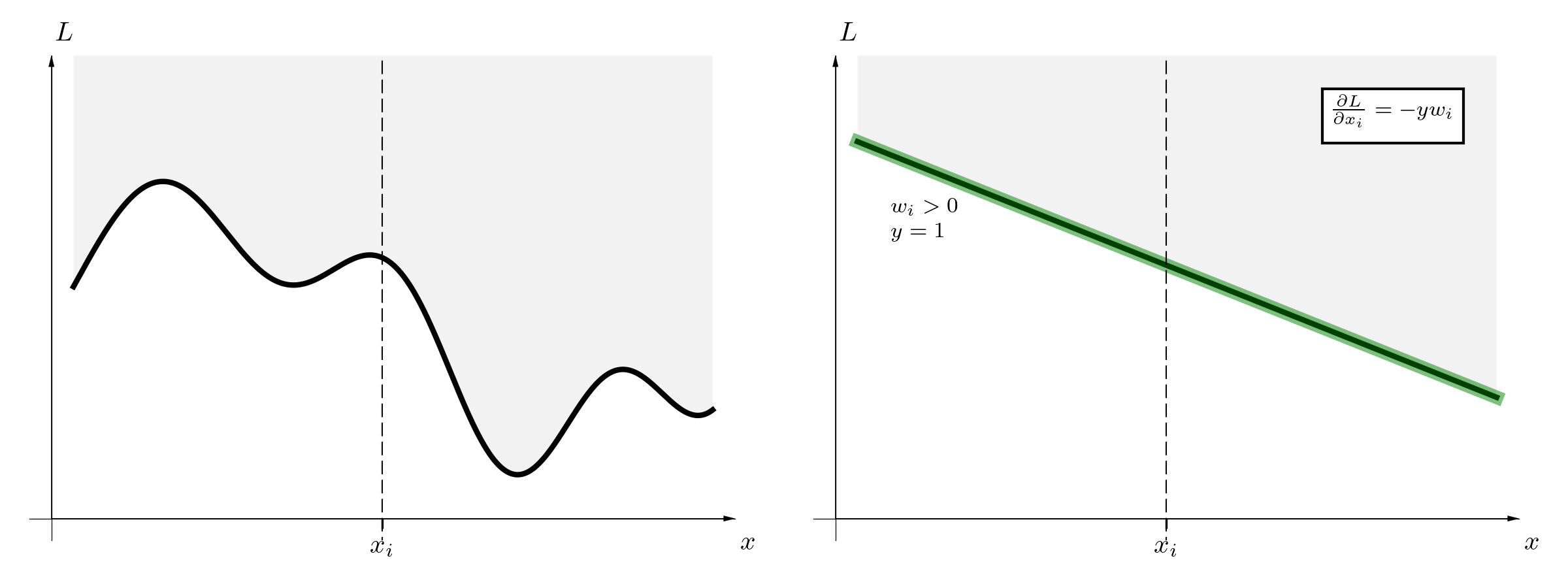
For our experiment, we use a simple linear classifier, so the model has only a single vector \(w\) and bias \(b\). The landscape of loss in terms of \(x_i\) for non-linear models is highly irregular (left figure), however in our case, it is just a straight line (right figure).
Using a dataset and an optimization method gradient descent, we follow the gradient and look for the model parameters, which minimize the loss function:
\[\min_{w,b} \frac{1}{D} \sum_{(x,y) \in D} L (y \cdot (w^Tx + b))\]Super straightforward, right? This is our regular training. We minimize the expected value of the loss. Therefore, the model is looking for any (even weak) correlations, which improve the performance on average(no matter how disastrous its predictions sometimes are).
\[\min_{\theta} \underset{(x,y) \in D} {\mathbb{E}} \ell ( h_{\theta}(x), y )\]Towards Robust Binary Classification
As we mentioned in the introduction, ML models (deep neural networks in particular) are sensitive to small changes. Therefore now, we allow the input to be perturbed a little bit. We are not interested in patterns which concern \(x\) exclusively but the delta neighbourhood around \(x\). In consequence, we face the min-max problem, and two related challenges.
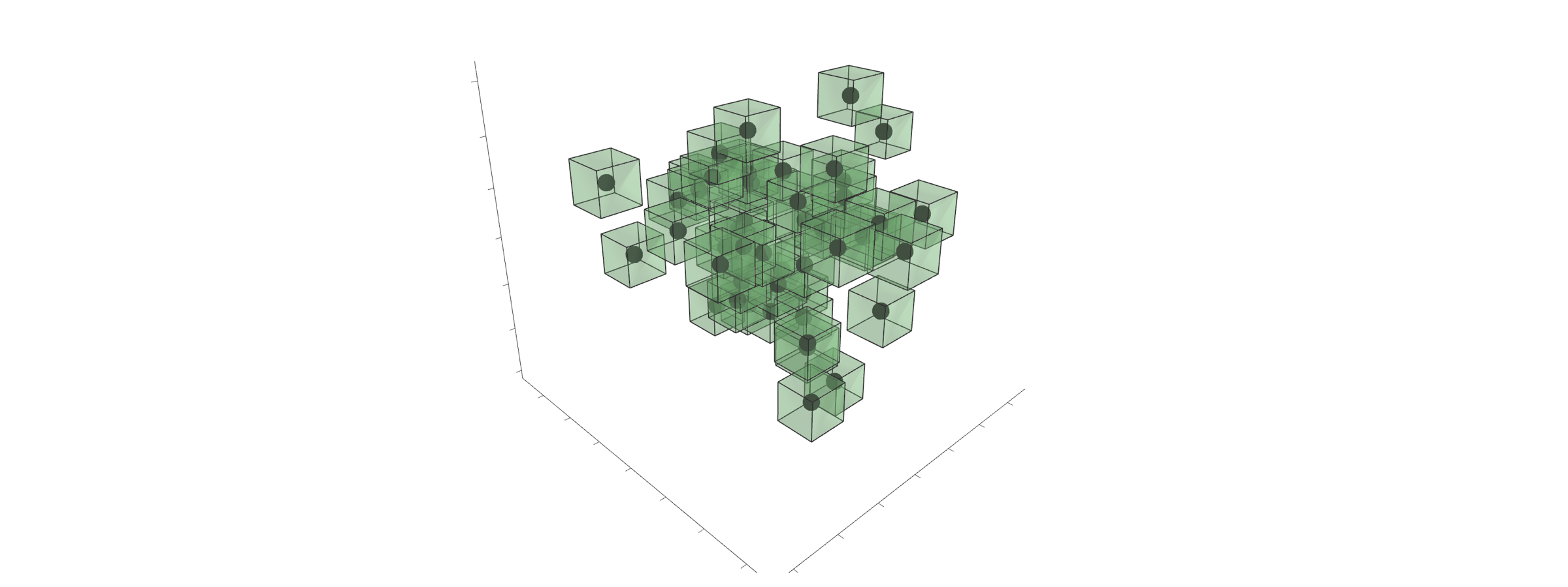
\[\min_{w,b} \frac{1}{D} \sum_{(x,y) \in D} \max_{\delta \in \Delta} L (y \cdot (w^T(x+ \delta) + b))\]Firstly, how can we construct valid perturbations \(\Delta\)? We want to formulate a space (epsilon-neighbourhood) around \(x\) (figure below), which sustains human understanding about this space. In our case, if a point \(x\) describes the digit one, then we have to guarantee that each perturbation \(x+\delta\) looks like the digit one. We do not know how to do this formally. However, we can (sure enough) assume that the small norm perturbations are correct \(\Delta = \{ \delta : || \delta || \leq \epsilon \}\). In our experiments, we are using the infinity norm \(|| \cdot ||_\infty\) (others are common too). These tiny boxes are neat, because valid perturbations are in the range \(−\epsilon\) to \(\epsilon\), independent of dimension.
The second challenge is how to solve the inner maximization problem. Most advanced ML models are highly non-linear, so this is tough in general. There are several methods to approximate the solution (a lower or upper bound), which we are going to cover in upcoming blog posts. Hopefully, in the linear case, we can easily solve this exactly because the loss directly depends on \(x\), our simplified loss landscape (formal details here).
\[\min_{w,b} \frac{1}{D} \sum_{(x,y) \in D} L \left(y \cdot (w^Tx + b) − \epsilon \|w\|_1 \right )\]The basic intuition is that we do not penalize high weights, which are far from the decision boundary (in contrast to regularization \(L_1\)). However, this is far from a complete explanation.
Firstly, the loss does not penalize if a classifier makes a mistake that is close to the decision boundary (left figure). The error tolerance dynamically changes with regards to model weights, shifting the loss curve. As opposed to regular training, we do not force a strictly defined margin to be preserved, which sometimes can not be achieved.

Secondly, the back propagation is different (right figure). The gradient is not only diminished, but also if it is smaller than epsilon, it can even change the sign. As a result, the weights that are smaller than epsilon are gently wiped off.
Finally, our goal is to minimize the expected value of the loss not only of input \(x\), but the close neighbourhood around \(x\):
\[\min_{w,b} \frac{1}{D} \sum_{(x,y) \in D} \mathbb{E} \left[ \max_{\delta \in \Delta} \ell ( h_{\theta}(x), y ) \right]\]Experiments
As we have already mentioned, today, we are doing a simple binary classification. Let’s briefly present regular training. We reduce the MNIST dataset to include exclusively only the digits zero and one (transforming the original dataset here). We build a regular linear classifier, SGD optimizer, and hinge loss. We work with the high-level Keras under Tensorflow 2.0 with eager execution (PyTorch alike).
# Convert Multi-class problem to binary
train_dataset = data.binary_mnist(split='train').batch(100)     # In fact, we should do three folded split
test_dataset = data.binary_mnist(split='test').batch(1000)      # to make a valid test.

# Build and compile linear model
model = keras.Sequential([
    keras.layers.Flatten(input_shape=(28, 28, 1)),
    keras.layers.Dense(1),
])
sgd_optimizer = keras.optimizers.SGD(learning_rate=.1)
hinge_loss = keras.losses.Hinge()  # This is: max(0, 1 - y_true * y_pred), where y_true in {+1, -1}
In contrast to just invoking the built-in fit method, we build the custom routine
to have full access to any variable or gradient.
We abstract the train_step, which processes a single batch.
We build several callbacks to collect partial results for further analysis.
def train_step(inputs, targets):        # Inject dependencies: a model, loss, and an optimizer
    with tf.GradientTape() as tape:
        prediction = model(inputs)
        loss_value = hinge_loss(prediction, targets)
    gradients = tape.gradient(loss_value, model.trainable_variables)
    sgd_optimizer.apply_gradients(zip(gradients, model.trainable_variables))
    predicted_labels = tf.sign(prediction)
    return predicted_labels, loss_value, gradients
The robust training is similar. The crucial change is the customized loss, which contains additionally \(− \epsilon \|w\|_1\) term.
def robust_hinge_loss(model, y_hat, y):     # Inject the epsilon
    w, b = model.trainable_variables
    hinge = lambda x: tf.maximum(0, 1-x)    # The raw hinge function
    delta = -epsilon * tf.norm(w, ord=1)    # Use the inf ball
    z1 = y * tf.reshape(y_hat, [-1])
    z2 = tf.add(z1, delta)
    loss_value = hinge(z2)
    return loss_value
Results
We do a binary classification to recognize the digits zero and one from the MNIST dataset. We train regular and robust models using presented scripts (1, 2). Our regular model achieves super results (robust models are slightly worse).

We have only single mistakes (figure below). A dot around a digit causes general confusion. Nevertheless, we have incredibly precise classifiers. We have achieved human performance in recognizing handwritten digits zero and one, haven’t we?

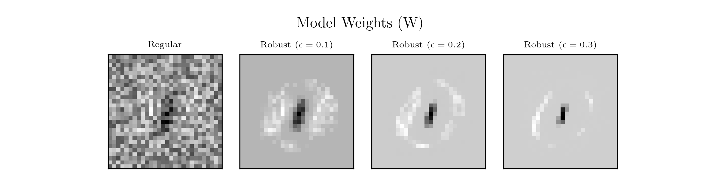
Not really. We can precisely predict (without overfitting, take a look at the tiny gap between the train and the test results), that’s all. We are absolutely far from human reasoning when it comes to recognizing the digits zero and one. To demonstrate this, we can check the model weights (figure below). Our classifiers are linear therefore the reasoning is straightforward. You can imagine a kind of a single stamp. The decision moves toward the digit one if black pixels are activated (and to the digit zero if white). The regular model contains a huge amount of weak features, which do not make sense for us, but generalize well. In contrast, robust models wipe out weak features (which are smaller than epsilon), and stick with more robust and human aligned features.
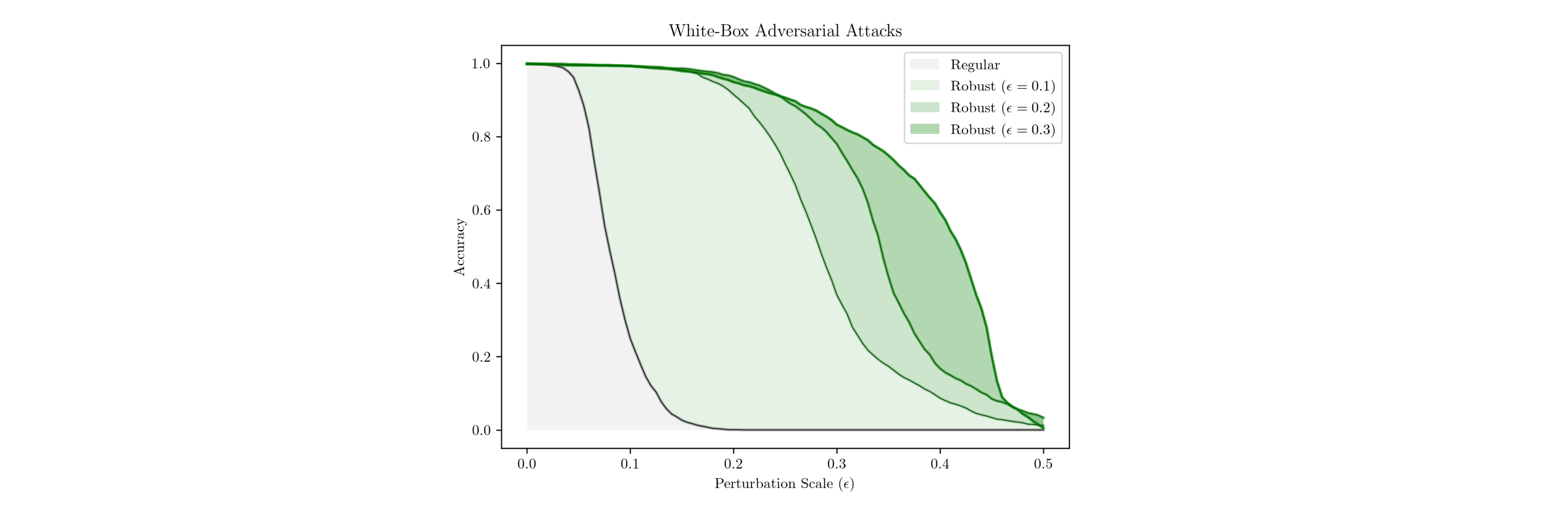
Now, we will make several white-box adversarial attacks and try to fool our models. We evaluate the models on perturbed test datasets, in which each sample is moved directly towards a decision boundary. In our linear case, the perturbations can be easily defined as:
\[\delta^\star = − y \epsilon \cdot \mathrm{sign}(w)\]where we check out several epsilons (figure below).
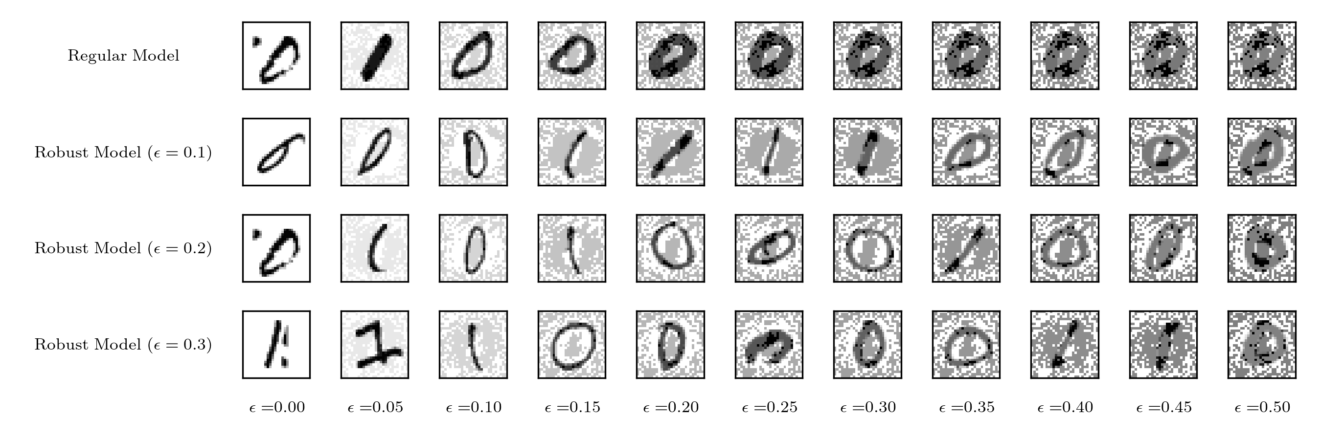
As we expect, the regular model is brittle due to the huge amount of weak features. Below, we present the misclassified samples which are closest to the boundary decision (predicted logits are around zero). Now, we can understand how perturbed images are so readable to humans e.g. \(\epsilon=0.2\) where the regular classifier has the accuracy around zero. The regular classifier absolutely does not know what the digit zero or one looks like. In contrast, robust models are generally confused about the different digit structures, nonetheless, the patterns are more robust and understandable to us.
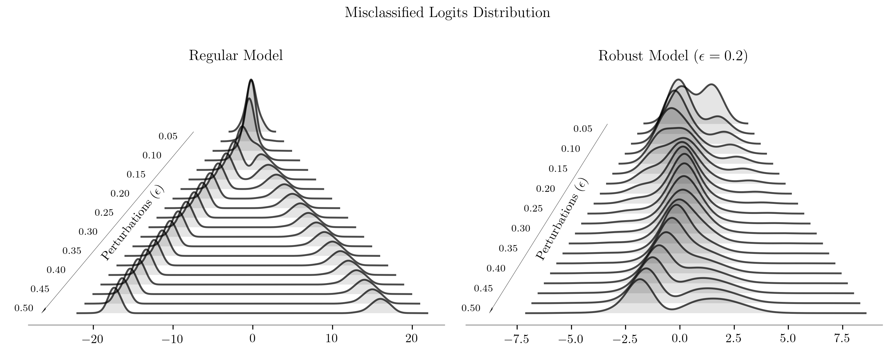
In the end, we present a slightly different perspective. Take a look at the logit distributions of misclassified samples. We see that the regular model is extremely confident about wrong predictions. In contrast, the robust model (even if it is fooled) is uncertain, because logits tend to be close to zero. Robust models seem to be more reliable (figure below).
Conclusions
Machine Learning models are great and powerful. However, the characteristics of regular training can lead to serious consequences in terms of the security and safety of deep neural networks in particular. In this blog post, we have shown what simple robust training can look like. This is only a simple binary case, which (we hope) gives more intuition about the drawbacks of regular training, and shows why these problems are so vital. Of course, things are more complex if we want to force deep neural networks to be more robust because performance rapidly declines, and models become useless. Nonetheless, the ML community is working hard to popularize and develop the idea of a robust ML, as this blog post has tried to do.
References
Must read articles are listed in Adversarial Machine Learning Reading List (Nicholas Carlini)
Tutorials:
- CS231n: Adversarial Examples and Adversarial Training - Stanford, Ian Goodfellow
- Adversarial Robustness, Theory and Practice, MIT and video
- Adversarial Machine Learning - Part 1 and Part 2 Biggio Battista
Blog posts:
- A Brief Introduction to Adversarial Examples, Gradient Science Group MIT - Jul 2018
- Training Robust Classifiers - Part 1 and Part 2, Gradient Science Group MIT - Aug 2018
- Breaking things is easy, Ian Goodfellow and Nicolas Papernot - Dec 2016
- Is attacking machine learning easier than defending it? Ian Goodfellow and Nicolas Papernot - Feb 2017
- How to know when machine learning does not know, Nicolas Papernot and Nicholas Frosst - May 2019
- Why Machine Learning is vulnerable to adversarial attacks and how to fix it, KDnuggets - Jun 2019
- Breaking neural networks with adversarial attacks, KDnuggets - Mar 2019
- Adversarial Patch on Hat Fools SOTA Facial Recognition, Medium - Aug 2019
- Why deep-learning AIs are so easy to fool? Nature - Oct 2019
- “Brittle, Greedy, Opaque, and Shallow”: The Promise and Limits of Today’s Artificial Intelligence - A Conversation with Rodney Brooks and Gary Marcus (MIT) - Sep 2019
- Identifying and eliminating bugs in learned predictive models, DeepMind- Mar 2019
- Better Language Models and Their Implications, OpenAI - Feb 2019
Tools:
- MadryLab/robustness - library for experimenting with adversarial robustness
- CleverHans - library to benchmark machine learning systems’ vulnerability to adversarial examples
- Adversarial Robustness 360 Toolbox, IBM
Groups
- Robust ML (Maintainers MIT)
- Trusted AI Group IBM
- SafeAI ETH Zurich
Original publication is here.