Do You Trust in Aspect-Based Sentiment Analysis? Testing and Explaining Model Behaviors

This article aims to highlight the need for testing and explaining model behaviors. I’ve published an open-source aspect_based_sentiment_analysis package where the key idea is to build a pipeline which supports explanations of model predictions. I’ve introduced an independent component called the professor that supervises and explains model predictions. Although we can benefit from explanations to understand individual predictions, we can also infer general characteristics of model reasoning what enhances control over the model. I truly believe that testing and explaining model behaviors can fuel further development, and make models more useful within real-world applications.

import aspect_based_sentiment_analysis as absa

recognizer = absa.aux_models.BasicPatternRecognizer()
nlp = absa.load(pattern_recognizer=recognizer)
completed_task = nlp(text=..., aspects=['slack', 'price'])
slack, price = completed_task.examples

absa.summary(slack)
absa.display(slack.review)

Introduction

Natural Language Processing is in the spotlight at the moment. This is mainly due to the stunning capabilities of modern language models. They can transform text into meaningful vectors that approximate human understanding of text. As a result, computer programs can now analyze texts (documents, mails, tweets etc.) roughly the same as people do. Extreme power of modern language models has fueled the NLP community to build many other, more specialized models that aim to solve specific problems, for example, sentiment classification. The community has built up open-source projects that provide easy access to countless finely-tuned models. Unfortunately, the usefulness of the majority of them is questionable when it comes to real-world applications.

ML models are powerful because they approximate the desired transformation, mapping between inputs and outputs, directly from the data. By design, the model collects any correlations in the data that are useful for making the correct mapping. This simple restriction-free rule forms the complex model reasoning that enables approximation of any logic behind the transformation. This is the big advantage of ML models, especially in cases in which the transformation is intricate and vague. However, this restriction-free process of forming model reasoning can also be a major headache because it can be problematic when it comes to keeping control of the model.

It is hard to force any model to capture a general problem (e.g. sentiment classification) solely by asking it to solve a specific task, a common evaluation task (e.g. SST-2) or a custom-built task based on labeled (sampled from production) data. This is because the model discovers any useful correlations, no matter they describe a general problem well and make sense to human beings or whether they are just exclusively effective in solving a specific task. Unfortunately, this second group of adverse correlations that encode dataset specifics can cause unpredictable model behavior on data that may be even just slightly different than used in a training. Due to this unfortunate nature of ML models, it is important to test how a model behavior is consistent with expected behavior. This is crucial because a model working in a real-world application is exposed to process data that is changing in time.

Before serving a model, the bottom line is to form valuable tests (so called sanity checks) that confirm whether the model reasoning satisfied our expectations or not. As a result, the model that meets test conditions is stable in test boundaries at least. Note that it is unknown what is beyond the test boundaries. Unfortunately, as long as neural networks form reasoning without restrictions, we cannot be sure that the model will behave according to our expectations in every case. Nonetheless, the risk of unexpected behavior can and should be minimized.

The sanity checks assure us that the model is working properly at the time of the deployment. Commonly, performance starts decline in time so it’s vital to monitor the model once it’s served. It is hard to track unexpected model behaviors having only a prediction, therefore, the proposed in this article pipeline is enriched by an additional component called the professor. The professor reviews model internal states, supervises the model, and provides explanations of model predictions that help to reveal suspicious behaviors. The explanations not only give us more control over the served model but also enhance further development. The analysis of explanations can lead to the formation of newer more demanding tests that force a model to improve.
I believe that both testing and explaining model behaviors are important in building production-ready stable ML models. This is especially important in cases wherein a huge model is fine-tuned on a modest dataset because, due to the nature of ML models, we have problems to define the desired task precisely. This is a fundamental problem among many down-stream NLP tasks but, in this article, we focus on aspect-based sentiment classification.

Definition of the Problem

The aim is to classify the sentiments of a text concerning given aspects. I have made several assumptions to make the service more helpful. Namely, the text being processed might be a full-length document, the aspects could contain several words (so may be defined more precisely), and most importantly, the service provides an approximate explanation of any decision made, therefore, a user is able to immediately infer the reliability of a prediction.

import aspect_based_sentiment_analysis as absa

nlp = absa.load()
text = ("We are great fans of Slack, but we wish the subscriptions "
        "were more accessible to small startups.")

slack, price = nlp(text, aspects=['slack computer program', 'price'])
assert price.sentiment == absa.Sentiment.negative
assert slack.sentiment == absa.Sentiment.positive

Above is an example of how quickly you can start to benefit from the open-source package. All you need is to do is to call the load function which sets up the ready-to-use pipeline nlp. You can explicitly pass the model name you wish to use (a list of available models is here), or a path to your model. In spite of the simplicity of using fine-tune models, I encourage you to build a custom model which reflects your data. The predictions will be more accurate and stable, something which we will discuss later on.

Pipeline: Keeping the Process in Shape

The pipeline provides an easy-to-use interface for making predictions. Even a highly accurate model will be useless if it is unclear how to correctly prepare the inputs and how to interpret the outputs. To make things clear, I have introduced a pipeline (that is closely linked to a model). It is worth to know how to deal with the whole process, especially if you plan to build a custom model.

The diagram above illustrates an overview of the pipeline stages. As usual, at the very beginning, we pre-process the raw inputs. We convert the text and the aspects into a task which keeps examples (pairs of a text and an aspect) that we can then further tokenize, encode and pass to the model. The model makes a prediction, and here is a change. Instead of directly post-processing the model outputs, I have added a review process wherein the independent component called the professor supervises and explains a model prediction. The professor might dismiss a model prediction if the model internal states or outputs seem suspicious. In the next sections, we will discuss in detail how the model and the professor work.

import aspect_based_sentiment_analysis as absa

name = 'absa/classifier-rest-0.2'
model = absa.BertABSClassifier.from_pretrained(name)
tokenizer = absa.BertTokenizer.from_pretrained(name)
professor = absa.Professor(...)     # Explained in detail later on.
text_splitter = absa.sentencizer()  # The English CNN model from SpaCy.
nlp = absa.Pipeline(model, tokenizer, professor, text_splitter)

# Break down the pipeline `call` method.
task = nlp.preprocess(text=..., aspects=...)
tokenized_examples = nlp.tokenize(task.examples)
input_batch = nlp.encode(tokenized_examples)
output_batch = nlp.predict(input_batch)
predictions = nlp.review(tokenized_examples, output_batch)
completed_task = nlp.postprocess(task, predictions)

Above is an example how to initialize the pipeline directly, and we revise in code the process being discussed by exposing what calling the pipeline does under the hood. We have omitted a lot of insignificant details but there’s one thing I would like to highlight. The sentiment of long texts tends to be fuzzy and neutral. Therefore, you might want to split a text into smaller independent chunks, sometimes called spans. These could include just a single sentence or several sentences. It depends on how the text_splitter works. In this case, we are using the SpaCy CNN model, which splits a document into single sentences, and, as a result each sentence can then be processed independently. Note that longer spans have richer context information, so a model will have more information to consider. Please take a look at the pipeline details here.

Model: Heart of the Pipeline

The core component of the pipeline is the machine learning model. The aim of the model is to classify the sentiment of a text for any given aspect. This is challenging because sentiment is frequently meticulously hidden. Nonetheless, before we jump into the model details, we will look more closely into how we have approached this task in the past, what the language model is, and why it makes a difference.

The model is a function that maps input to a desired output. Because this function is unknown, we try to approximate it using data. It is hard to build a dataset that is clean and big enough (for NLP tasks in particular) to train a model directly in a supervised manner. Therefore, the most basic approach to solving this problem, and to overcoming the lack of a sufficient amount of data, is to construct hand-crafted features. Engineers extract key tokens, phrases, n-grams, and train a classifier to assign weights on how likely these features are to be either positive, negative or neutral. Based on these human-defined features, a model can then make predictions (that are fully interpretable). This is a valid approach, pretty popular in the past. However, such simple models cannot precisely capture complexity of the natural language, and as a result, they can quickly reach the limit of their accurateness. This is a problem which is hard to overcome.

We made a breakthrough when we started to transfer knowledge from language models to down-stream, more specific, NLP tasks. Nowadays, it is a standard that the key component of the modern NLP application is the language model. Briefly, a language model gives a rough understanding of natural language. In computational heavy training, it processes enormous datasets, such as the entire Wikipedia or more, to figure out relationships between words. As a result, it is able to encode words, meaningless strings, into rich in information vectors. Because encoded-words, context-aware embeddings, are living in the same continuous space, we can manipulate them effortlessly. If you wish to summarize a text, for example, you might sum vectors; compare two words, make a dot product between them, etc. Rather than using feature engineering, and the linguistic expertise of engineers (implicit knowledge transfer), we can benefit from the language model as a ready-to-use, portable, and powerful features provider.

Within this context, we are ready to define the SOTA model, which is both powerful and simple. The model consists of the language model bert, which provides features, and the linear classifier. From among variety of language models, we use BERT, because we can benefit directly from BERT’s next-sentence prediction to formulate the task as a sequence-pair classification. As a result, an example is described as one sequence in the form: [CLS] text subtokens [SEP] aspect subtokens [SEP]. The relationship between a text and an aspect is encoded into the [CLS] token. The classifier just makes a linear transformation of the final special [CLS] token representation.

import transformers
import aspect_based_sentiment_analysis as absa

name = 'absa/bert_abs_classifier-rest-0.1'
model = absa.BertABSClassifier.from_pretrained(name)
# The model has two essential components:
#   model.bert: transformers.TFBertModel
#   model.classifier: tf.layers.Dense 

# We've implemented the BertABSClassifier to make room for further research.
# Nonetheless, even without installing the `absa` package, you can load our 
# bert-based model directly from the `transformers` package.
model = transformers.TFBertForSequenceClassification.from_pretrained(name)

Even if it is rather outside the scope of this article, note how to train the model from scratch. I started with the original BERT version as a basis, and I divided the training into two stages. Firstly, due to the fact that BERT is pretrained on dry Wikipedia texts, I biased the language model towards more informal language (or a specific domain). To do this, I’ve selected raw texts close to the target domain and have done a self-supervised language model post-training. The routine is the same as the pre-training but you need to carefully set up the optimization parameters. Secondly, I did regular supervised training. I trained the whole model jointly, the language model and the classifier, using a fine-grained labeled dataset. There are more details about the model here and training here.

Awareness of the Model Limitations

In the previous section, I presented an example of a modern NLP architecture wherein the core component is a language model. We abandoned task specific and time consuming feature engineering. Instead, thanks to language models, we can use powerful features, context-aware word embeddings. Nowadays, transferring knowledge from language models has become extremely popular. This approach dominates the leader boards of any NLP task, including aspect-based sentiment classification (see the table below). Nonetheless, we should interpret these results with caution.

A single metric might be misleading, especially when the evaluation dataset is modest (as in this case). According to the introduction, a model seeks any correlations it deems useful for making a correct prediction, regardless of whether they make sense to human beings or not. As a result, model reasoning and human reasoning are very different. A model encodes dataset specifics invisible to humans. In return for the high accuracy of massive modern models, we have little control over the model behavior - because both the model reasoning and the dataset characteristics which the model is trying to map precisely, are unclear. It is a serious problem because during an inference, unconsciously exposing a model to examples which are completely unusual is much more likely, and this can cause unpredictable model behavior. To avoid such dangerous situations and to better understand what is beyond the comprehension of a model, we need to construct additional sanity checks; fine-grained evaluations.

In the table below, I present three exemplary tests that roughly estimate model limitations. To be consistent, I examine the BERT-ADA model introduced in the previous section. Test A checks how crucial the information about an aspect is. I limit the model to predict sentiment without providing any aspects. The task then becomes a basic, aspect independent, sentiment classification (details are here). Test B verifies how a model considers an aspect. I force a model to predict using unrelated aspects (instead of the correct ones); manually selected and verified simple nouns that are not present in the dataset, even implicitly. I process positive and negative examples, expecting to get neutral sentiment predictions (details are here). Test C examines how precisely a model separates information about a requested aspect from other aspects. In the first case, I process positive and neutral examples wherein I add to texts a negative emotional sentence about a different aspect. For instance, “The {other aspect} is really bad.” expecting that the model will persist in making its predictions, without any changes. In the second case, I process negative and neutral examples with an additional positive sentence “The {other aspect} is really great.”. In both cases, I use hand-crafted templates and verified unrelated aspects from test B (details are here).

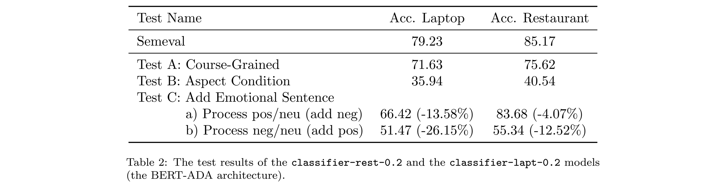
Test A confirms that the course-grained classifier is achieving good results as well (without any adjustments). This is not good news. If a model predicts a sentiment correctly without taking into account an aspect, roughly, there will be no gradient towards patterns that support aspect-based classification, and the model will have nothing to improve in this direction. Consequently, at least 70% of the already limited dataset will not help to improve the aspect-based sentiment classification. In addition, these examples might even be disruptive, because they could overwhelm examples which require multi-aspect consideration. Multi-aspect examples might become treated as outliers, and gentle erased due to averaging of a gradient in a batch for example (the test summary is here).

Test B demonstrates that a model may not truly solve aspect-based conditions, because it considers an aspect mainly as a feature, not as a constraint. In 35 and 40% of cases, a model recognizes correctly that the text does not concern a given aspect, and returns a neutral sentiment instead of positive or negative. The model’s accurateness in terms of aspect-based classification is questionable. One might conclude this directly from the model architecture because there is no dedicated mechanism that might impose the aspect-based condition (the test summary is here).

Test C shows that a model separates information about different aspects well. The reference is given in brackets to emphasize how enriched texts decrease model performance of processing a) positive/neutral and b) negative/neutral examples. In most cases, the model correctly deals with a basic multi-aspect problem, and recognizes that an added sentence, highly emotional in the opposite direction, does not concern a given aspect. Even if test B shows that the model is neglecting in some cases information about an unrelated aspect, this test reveals that an aspect is a really vital feature if a text concerns many aspects including the given aspect, and the model needs to separate out information about different aspects (the test summary is here).

The model behavior tests, as shown above, can provide many valuable insights. Unfortunately, papers describing state-of-the-art models quietly ignore tests that may expose model limitations. In contrast, I encourage you to do those tests. Even though they might be time-consuming and tedious, test-driven model development is powerful because you can understand any model defects in detail, fix them, and make further improvements more smoothly.

The Professor: Supervising Model Predictions

The tests so far performed have exposed some model limitations. The most natural way to eliminate these would be to fix the model itself. Firstly, keeping in mind that a model reflects the data, we could augment a dataset, and add examples that the model has difficulties with predicting correctly. Since manual labeling is time-consuming, we might think about generating examples. Nonetheless, models adapt quickly to fixed structures, so the benefits might be minimal. Secondly, of course, we could propose a new model architecture. This is an appealing direction from the perspective of a researcher, however, profits from the findings are uncertain.

Due to problematic model fixing, unknown model reasoning, and limited decision control, I have abandoned the idea of using a standard pipeline that relies exclusively on a single end-to-end model. Instead, before making a final decision, I fortify the pipeline with a reviewing process. I introduce a distinct component - the professor - to manage the reviewing process. The professor reviews the model’s hidden states and outputs, to both identify and correct suspicious predictions. It is composed of either simple or complex auxiliary models that examine the model reasoning and correct any model weaknesses. Because the professor takes into account information from aux. models in order to make the final decision, we have greater control over the decision-making process, and we can freely customize the model behavior.

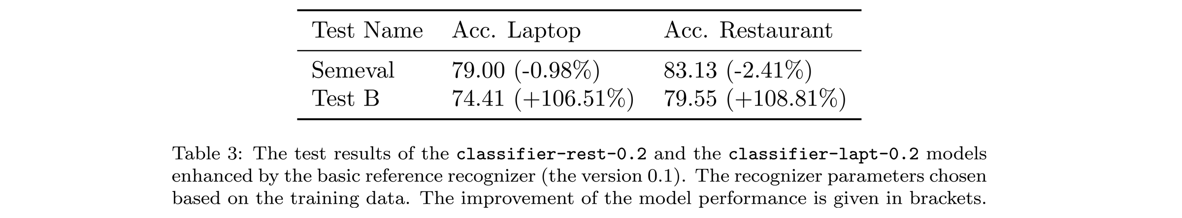
The Professor: Fixing Model Limitations

Firstly, I highlight how to start fixing the model limitations more smoothly using the professor. Coming back to the problem stated in test B, avoiding questionable predictions, we want to build an aux. classifier that predicts whether a text relates to an aspect or not. If there is no reference in a text to an aspect, the professor sets a neutral sentiment regardless of the model prediction (details are here).

import aspect_based_sentiment_analysis as absa

name = 'absa/basic_reference_recognizer-rest-0.1'
recognizer = absa.aux_models.BasicReferenceRecognizer.from_pretrained(name)
professor = absa.Professor(reference_recognizer=recognizer)

Good practice is to gradually increase the model complexity in response to demands. I propose a simple aux. model BasicReferenceRecognizer for now that only checks if an aspect is clearly mentioned in a text (model details are here, the training is here). The table below confirms the significant improvement of Test B performance. Nonetheless, in most cases, there is a trade-off between the performance of different tests as it is here. Note that this is a simple test case. Therefore, I encourage you to construct more challenging tests wherein aspect mentions are more implicit.

The Professor: Explaining Model Reasoning

There is a second, more important reason why we have introduced the professor. The professor’s main role is to explain model reasoning, something which is extremely hard. We are far from explaining model behavior precisely even though it is crucial for building intuition to fuel further research and development. In addition, model transparency enables an understanding of model failures from various perspectives, such as safety (e.g. adversarial attacks), fairness (e.g. model biases), reliability (e.g. spurious correlations), and more.

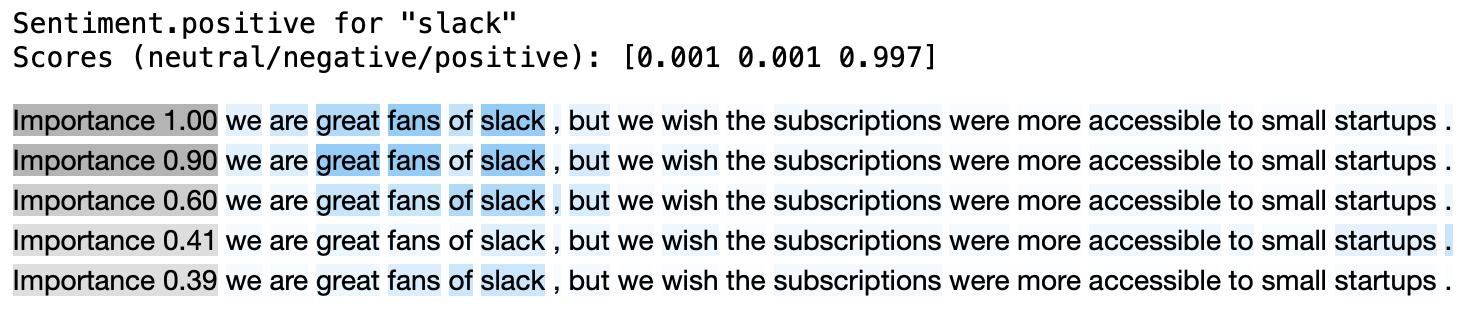
Explaining model decisions is challenging, but not only due to model complexity. As we mentioned before, models make decisions in a completely different way to people. We need to translate abstract model reasoning into a form understandable for humans. To do so, we have to break down model reasoning into components that we can understand. These are called patterns. A pattern is interpretable and has an importance attribute (within the range <0, 1>) that expresses how a particular pattern contributes to the model prediction.

A single pattern is a weighted composition of tokens. It is a vector that assigns a weight for each token (within the range <0, 1>) that defines how a token relates to a pattern (an example below). For instance, a one-hot vector illustrate a simple pattern that is exclusively composed of a single token. This interface, the pattern definition, enables either simple or more complex relations to be conveyed. It can capture key tokens (one-hot vectors), key token pairs or more tangled structures. The more complex the interface (the pattern structure), the more details can be encoded. In the future, the interface of model explanation might be a natural language itself.

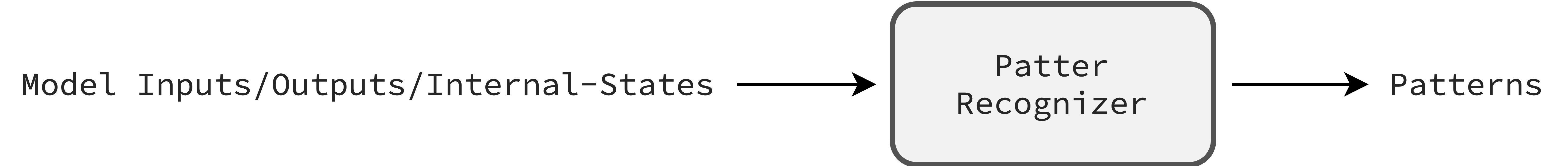
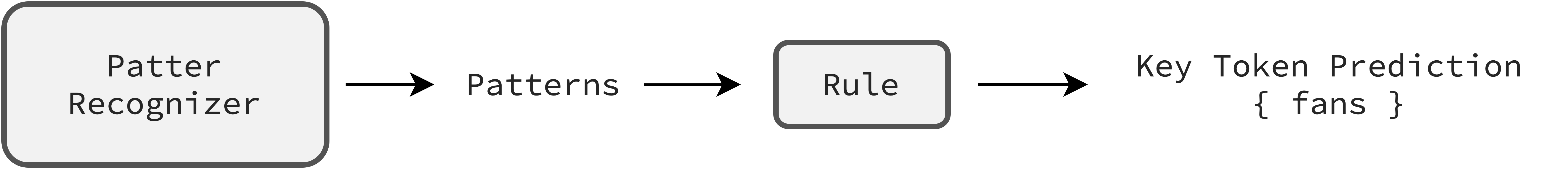
The key concept is to frame the problem of explaining a model decision as an independent task wherein an aux. model, the pattern recognizer, predicts patterns given model inputs, outputs, and internal states. This is a flexible definition, so we will be able to test various recognizers in the longer perspective. We can try to build model-agnostic pattern recognizer (independent with respect to the model architecture or parameters). We can customize inputs, for instance, take into account internal states or not, analyze a model holistically or derive conclusions from only a specific component. Finally, we can customize outputs, defining sufficient pattern complexity. Note that it is a challenge to design training and evaluation, because the true patterns are unknown. As a result, extracting complex patterns correctly is extremely hard. Nonetheless, there are a few successful methods to train a pattern recognizer that can reveal latent rationales. This is the case in which a pattern recognizer tries to mask-out as many input tokens as possible, constrained to keeping an original prediction (e.g. the DiffMask method).

Due to time constraints, at first I did not want to research and build a trainable pattern recognizer. Instead, I decided to start with a pattern recognizer that originates from our observations, prior knowledge. The model, the aspect-based sentiment classifier, is based on the transformer architecture wherein self-attention layers hold the most parameters. Therefore, one might conclude that understanding self-attention layers is a good proxy to understanding a model as a whole. Accordingly, there are many articles [ 1, 2, 3, 4, 5 ] that show how to explain a model decision in simple terms, using attention values (internal states of self-attention layers) straightforwardly. Inspired by these articles, I have also analyzed attention values (processing training examples) to search for any meaningful insights. This exploratory study has led me to create the BasicPatternRecognizer (details are here).

import aspect_based_sentiment_analysis as absa

# This pattern recognizer doesn't have trainable parameters
# so we can initialize it directly, without setting any weights. 
recognizer = absa.aux_models.BasicPatternRecognizer()   
professor = absa.Professor(pattern_recognizer=recognizer)

# Examine the model decision.
nlp = absa.Pipeline(..., professor=professor) # Set up the pipeline. 
completed_task = nlp(text=..., aspects=['slack', 'price'])
slack, price = completed_task.examples
absa.display(slack.review) # It plots inside a notebook straightaway.
absa.display(price.review)

Verification of Explanation Correctness

The explanations are only useful if they are correct. To form the basic pattern recognizer, I have made several assumptions (prior beliefs), therefore we should be careful about interpreting the explanations too literally. Even if the attention values have thought-provoking properties, for example, they encode rich linguistic relationships, there is no proven chain of causation. There are a lot of articles that illustrate various concerns why drawing conclusions about model reasoning directly from attentions might be misleading [ 1, 2, 3 ]. Even if the patters seem to be reasonable, the critical thinking is the key. We need a quantitative analysis to truly measure how correct the explanations are. Unfortunately, as with the training, the evaluation of a pattern recognizer is tough due to the fact that the true patterns are unknown. As a result, I am forced to validate only selected properties of the predicted explanations. Keeping this article concise, I cover solely two tests but there is much more to do to assess the reliability of explanations.

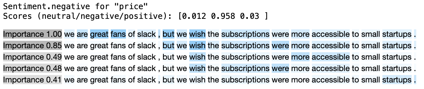
Verification of Explanation Correctness: Key Token Recognition Test

There are many properties needed to keep an explanation consistent and reliable but one is fundamental. The explanation should clearly indicate the most important (in terms of decision-making) token at least. To confirm whether the proposed BasicPatternRecognizer provides patterns that support this property or not, we can do a simple test (implementation is here).

We mask in a text the most important (according to patterns) token, and observe if the model changes the decision or not. The example might contain several key tokens, tokens that masked (independently) cause a change in the model’s prediction. The key assumption of this test is that the chosen token should belong to the group of key tokens if it is truly significant.

import aspect_based_sentiment_analysis as absa

patterns = ... # PredictedExample.review.patterns
key_token_prediction = absa.aux_models.predict_key_set(patterns, n=1)

It is important to be aware that the key token prediction comes from a pattern recognizer indirectly. We set up a plain rule predict_key_set (details are here) that sums the weighted (by importance values) patterns, and predicts a key token (in this case). Moreover, note that the test is simple and convenient because we are able to reveal valid key tokens (checking only n combinations at most) needed to measure the test performance precisely.

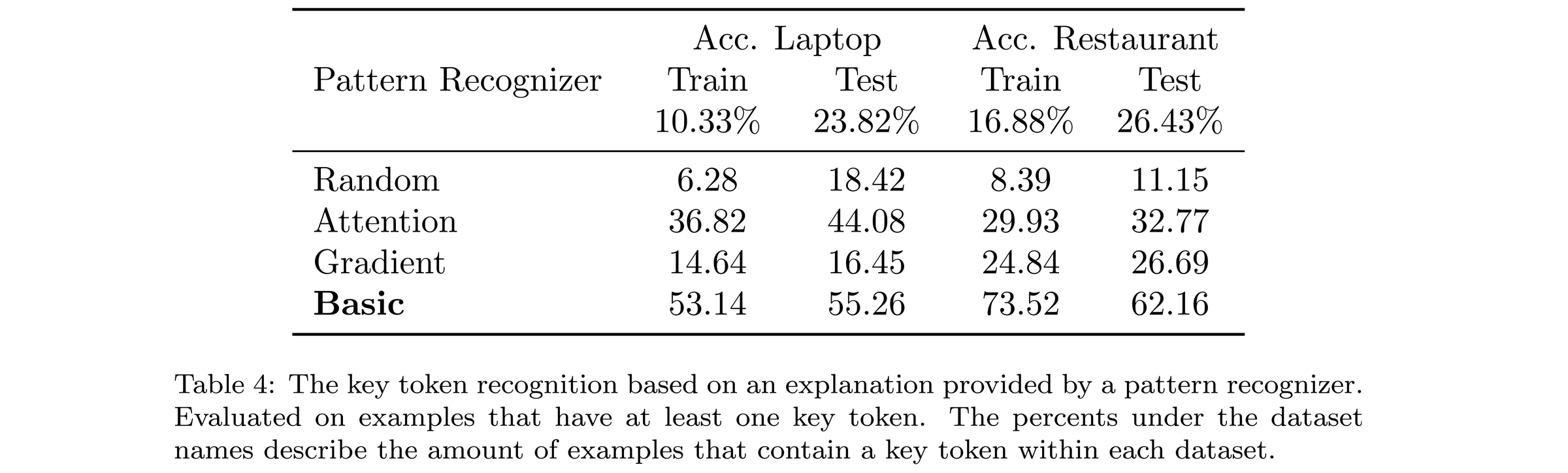
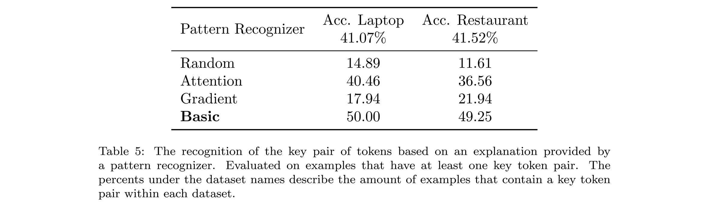
In the table above, I compare four pattern recognizers (details of other recognizers are here). For example, around 24% of the laptop test examples have at least one key token (others we filter out). Of those, around 55% of cases, the chosen token based on an explanation from the basic pattern recognizer is the key token. From this perspective, the basic pattern recognizer is more precise that other methods (more test results are here). It’s interesting that test datasets have significantly more examples that contain a key token. It suggests that model reasoning is different during processing known and unknown examples. In the next sections, we further analyse pattern recognizers solely on more reliable test datasets.

Verification of Explanation Correctness: Key Pair Recognition Test

The truth is that we cannot truly assess the correctness of explanations by evaluating only a single token. Therefore, to make this verification more reliable, we do a second similar test (implementation is here). The aim is to predict the key pair of tokens, a pair that masked causes a change in the model prediction.

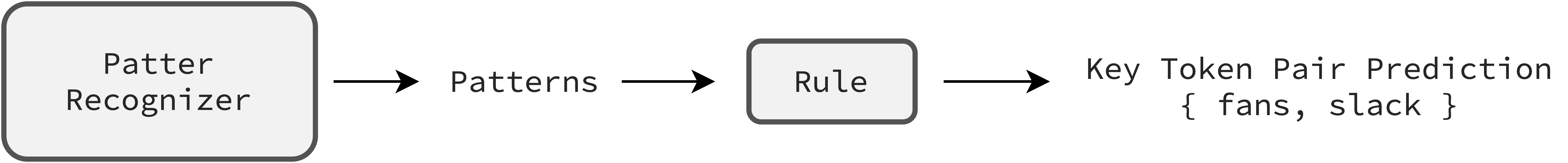
In the table below, I compare four pattern recognizers similarly as we have done in the previous test. For example, around 41% of the restaurant test examples have at least one key token pair (others we filter out). Of those, around 49% of cases, the chosen token pair from the basic pattern recognizer is the key pair of tokens. The basic basic pattern recognizer is still the most accurate but the advantage over other methods has been diminished. Note that this test covers the previous key token test, therefore, results are correlated.

Usually it is practically impossible to retrieve ground truth (existing too many combinations to check out), and this is the unfortunate implication of unknown model reasoning. We cannot say exactly how accurate pattern recognizers are (in most test cases) but still we can compare them. Below, we check the correctness of the basic pattern recognizer by comparing against other methods (the restaurant domain). This is the alternative approach of measuring the performance of a pattern recognizer.

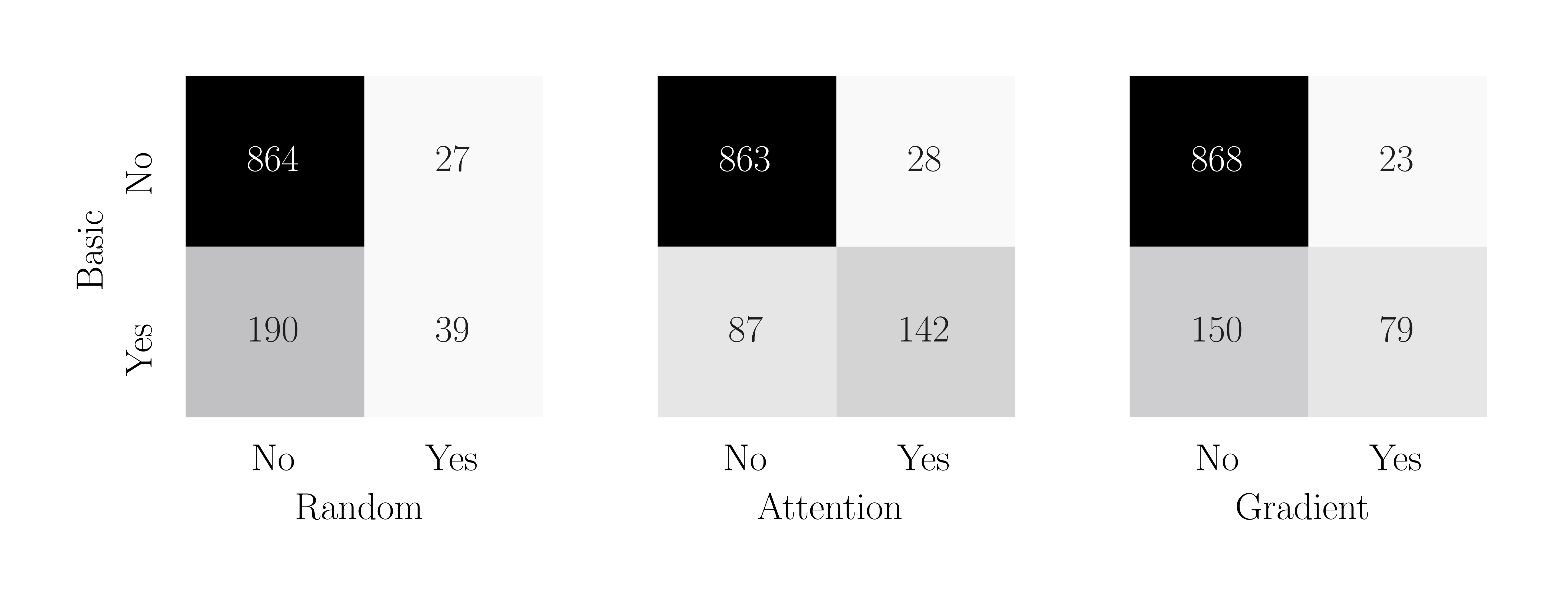
In matrices, on-diagonal values illustrate cases wherein recognizers behave similarly. In these cases, both recognizers choose a pair that masked either flips a model decision (the bottom-right cell) or does not (the upper-left cell). Off-diagonal values are more revealing because they expose differences. The bottom-left cell counts examples wherein the basic recognizer uncovers a key pair correctly while another recognizer does not, and the other way around (the upper-right cell). The upper-right value is also helpful to estimate how precise (at most) is the basic recognizer. To sum up, the basic recognizer aims to maximize the bottom-left and minimize the upper-right values. From this perspective as well, the basic pattern recognizer stands out from other methods (more test results are here).

Inferring from Explanations: Complexity of Model Reasoning

Building better pattern recognizers is not the sole goal (at least, not in this article). The aim is to benefit from a recognizer to be able to discover insights about a model (and a dataset), and use them to make improvements. For instance, the attractive information we can infer from explanations is the complexity of model reasoning. In this section, we investigate whether a single token usually triggers off a model or a model rather uses more sophisticated structures. The analysis may quickly reveal any alarming model behaviors because it is rather suspicious if a single token stands behind a decision of a neural network. Even though it might be a valuable study on its own, the key concept of this section is to give an example of how to analyse error-prone explanations as a whole, in contrast to reviewing them individually something which might be misleading.

Assuming (roughly) that more complex structures engage more tokens (e.g. more relationships potentially), we approximate the complexity of model reasoning by the number of tokens crucial to making a decision. We assume that crucial tokens are the minimal key set of tokens, the minimal set of tokens that masked (altogether) cause a change in the model’s prediction. As a result, we estimate the complexity using key sets that implicitly provide a pattern recognizer.

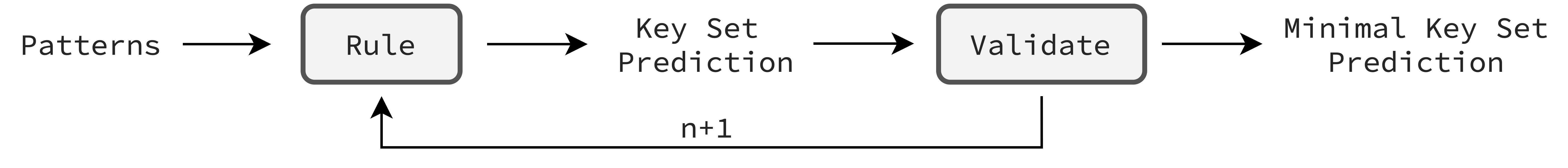
In this analysis, we benefit from the rule used in the last two tests that predicts (based on patterns) a key set of a given size n. To make this exemplary study clear, we want to be sure that analysing key sets are valid (causing a decision change). Therefore, I introduce a simple policy that includes a validation. Namely, starting with n=1, we iterate through key set predictions assuming that the first valid prediction is minimal. We validate a prediction by calling a model with the masked tokens (that belong to this set) expecting a decision change (implementation is here).

The chart below (on the left) presents the summary of model reasoning in terms of complexity. As we said, the complexity is approximated by the number of masked tokens needed to change the model’s decision. We infer them from patterns using a plain rule and policy. The plot presents model reasoning on restaurant test predicted-negative examples. Because the dataset is unbalanced (positive examples dominate), the model tends to classify masked examples as positive rather than neutral. This clearly demonstrates the confusion matrix on the right that keeps original sentiment predictions in rows, and sentiment predictions after masking in columns (using a key set that contains either one, two or three tokens chosen based on patterns provided by the basic pattern recognizer). Look at the second row of predicted negative examples. Many examples after masking change sentiment to positive. I investigate them and other positive predictions, and it turns out that almost fully masked examples remain positive. Therefore, the analysis of predicted-negative examples is more informative because predictions of positive sentiment would appear in the last column obscuring the overall picture. The problem occurs in both laptop and restaurant dataset domains (other plots are here).

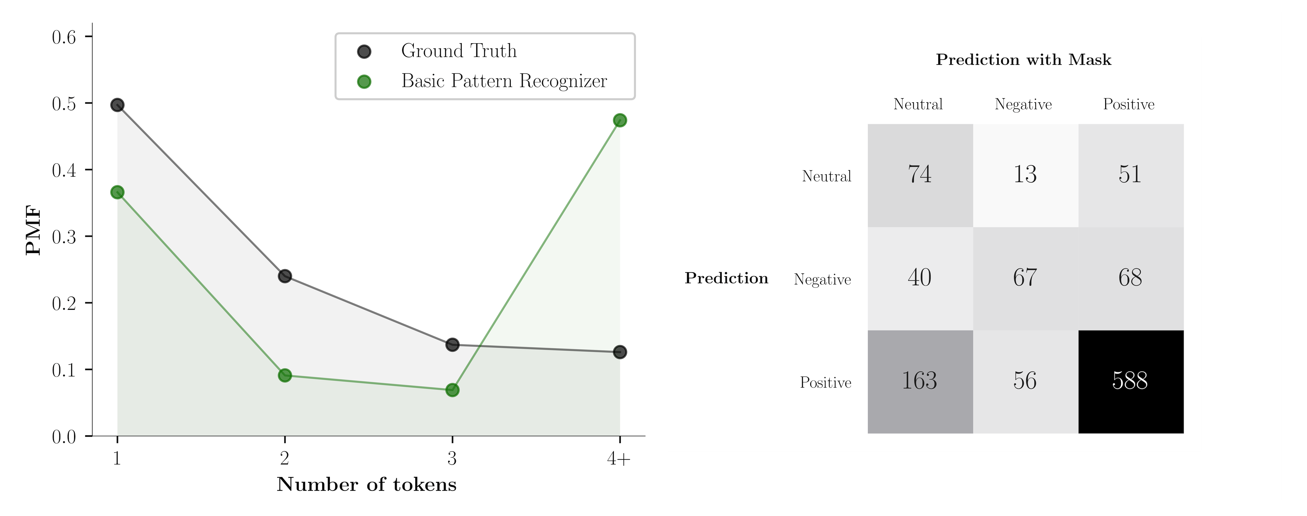
The decision in around 74% of cases is based on simple patterns wherein one or two masked tokens are enough to change a model’s prediction. The basic pattern recognizer provides rough understanding but it is far from being perfect. The last column shows that in 47% of cases it cannot find (misclassified) a valid key token set. Note that the ground truth is helpful but not crucial. The more precise recognizer would try to push the predicted distribution towards the left-hand side, therefore, without ground truth, still we can reveal valuable insights about model reasoning.

The analysis is done outside the pipeline (offline), to keep it clear. However, it can be easily adjusted to online monitoring of model behaviors. A key change concerns the number of additional calls to a model (preferably no calls). Instead of using a pain rule and policy, one can build another model that - based on patterns (or internal model states) - predicts whether an example has e.g. a key token or a key set of four tokens, without any extra calls to a model for verifications. As a result, the monitoring does not interfere with the model inference efficiency. The essence of this section is that we are able to track model behaviors e.g. complexity, and react if something goes wrong (or just changes rapidly).

Rolf: Exemplary Graphical User Interface

My superb colleagues have built ROLF, an exemplary GUI that demonstrates among other things the usefulness of approx. explanations (https://rolf.scalac.io). Without installing the package, you have a quick access to the default pipeline that the absa.load function returns. The backend solely wraps up a pipeline into the clear flask service which provides data to the frontend. Write your text, add aspects, and hit the button “analyze”. In a few seconds, you have a response, a prediction together with an estimated explanation. Please note that the service (unfortunately) is not updated to the newest version of the package.

Conclusions

The restriction-free process of creating model reasoning can build models that are both powerful and fragile at the same time. It is a big advantage that a model infers the logic behind the transformation directly from data. However, the discovered correlations (vague and intricate to human beings) can generalize well a given task but not necessarily a general problem. As a result, it is totally natural that a model behavior may not be consistent with the expected behavior.

This is a fundamental problem because adverse correlations that encode the task specifics can cause unpredictable model behavior on data even slightly different than that used in training. In contrast to SOTA models, a model working in a real-world application is exposed to data which changes in time. If we do not test and explain model behaviors (and do not fix model weaknesses), the performance of the served model can be unstable and will likely start to decline. And, it might be even hard to notice when a model is useless, and stops working at all (a distribution of predictions might remain unchanged).

In this article, I have highlighted the value of testing and explaining model behaviors. The tests can quickly reveal severe limitations of the SOTA model e.g. an aspect condition does not work as one might expect (works as a feature). We would be in troubles if we tried to use this model architecture in a real-world application. In general, it’s hard to trust model reliability if there is no tests that examine model behaviors, especially when a huge model is fine-tuned on a modest dataset (as it is with down-stream NLP tasks).

Testing assures us that the model works properly at the time of the deployment. It is worth to monitor the model once it’s served. The explanations of model decisions are extremely helpful to that end. We may benefit from explanations to understand an individual prediction but also to infer and monitor the general characteristics of model reasoning. Even rough explanations can help to recognize alarming behaviors. This article has given examples of how to have more control over the ML model. It is extremely important to keep an eye on model behaviors.

References

Introduction to the BERT interpretability:

• Analysis Methods in Neural Language Processing: A Survey (paper)
• Are Sixteen Heads Really Better than One? (paper)
• A Primer in BERTology: What we know about how BERT works (paper)
• What Does BERT Look At? An Analysis of BERT’s Attention (paper)
• Visualizing and Measuring the Geometry of BERT (paper)
• Is BERT Really Robust? A Strong Baseline for Natural Language Attack on Text Classification and Entailment (paper)
• Adversarial Training for Aspect-Based Sentiment Analysis with BERT (paper)
• Adv-BERT: BERT is not robust on misspellings! Generating nature adversarial samples on BERT (paper)
• exBERT: A Visual Analysis Tool to Explore Learned Representations in Transformers Models (paper)
• Does BERT Make Any Sense? Interpretable Word Sense Disambiguation with Contextualized Embeddings (paper)
• Attention is not Explanation (paper)
• Attention is not not Explanation (paper)
• Hierarchical interpretations for neural network predictions (paper)
• Analysis Methods in Neural NLP (paper)

How to use language models in the Aspect-Based Sentiment Analysis:

• Utilizing BERT for Aspect-Based Sentiment Analysis via Constructing Auxiliary Sentence (NAACL 2019) (paper)
• BERT Post-Training for Review Reading Comprehension and Aspect-based Sentiment Analysis (NAACL 2019) (paper)
• Exploiting BERT for End-to-End Aspect-based Sentiment Analysis (paper)